


🧾Introduction
One of the latest initiatives undertaken by the Rights Management team, was the migration of a legacy Django application to a more maintainable and scalable platform. The legacy application was reaching its limits and there was a real risk of missing revenue because the system could not handle any more clients.
To address this challenge, we developed a new platform that could follow the “deep pocket strategy.”
What does that mean for our team? Essentially, when the number of transactions we process spikes, we deploy as many resources needed in order to keep our SLAs.
With the end goal of building a platform capable of scaling, we decided to go with native cloud architecture and AsyncIO technologies. The first stress tests surprised (and baffled!) us, because the system didn’t perform as expected even for a relatively small number of transactions per hour.
This article covers our journey towards understanding the nuances of our changing architecture and the valuable lessons learned throughout the process. In the end (spoiler alert!) the solution was surprisingly simple, even though it took us on a profound learning curve. We hope our story will provide valuable insights for newcomers venturing into the AsyncIO world!
📖Background
Orfium’s Catalog Synchronization service uses our in-house built application called Rights Cloud. It’s tasked with managing music catalogs. Additionally, there’s another system, called Rights Manager, which handles synchronizing many individual catalogs with a user-generated content platforms (UGC,) such asYouTube.
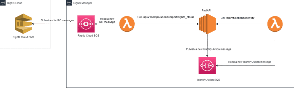
Every day, the Rights Manager system ingests Rights Cloud messages, which detail changes regarding a specific client’s composition metadata and ownership shares. For this, we had implemented the Fan-Out Pattern, so Rights Cloud sends the message to a dedicated topic (SNS) and then Rights Manager copies the message to its own queue (SQS). For every message that Rights Manager ingests successfully two things happen:
- The Rights Cloud composition is updated to the Rights Manager System. The responsible API is the Import Rights Cloud Composition
- After the successful Rights Cloud ingestion, a new action is created (delivery, update, relinquish). The API responsible for handling these actions is the Identify Actions API.
Based on this ingestion, the Rights Manager system then creates synchronization actions, such as new deliveries, update ownership shares, or relinquish.
Simplified Cloud Diagram of Rights Manager
😵The Problem
During our summer sprint, we rolled out a major release for our Rights Manager platform. After the release, we noticed some delays for the aforementioned APIs.
We noticed (see the diagrams below) spikes in latency between 10 to 30 seconds for the aforementioned APIs during the last two weeks of August.Even worse, some requests were dropped because of the 30-second web server timeout. Overall, the P90 latency was over 2 seconds. This was alarming, especially considering that the team had designed the system to meet a maximum latency performance metric of under 1 second.
We immediately started investigating this behavior because scalability is one of the critical aspects of the new platform.
First we examined the overall requests for the upper half of August.
At first glance, two metrics caught our attention:
- Alarming metric #1: The system could not handle more than ~78K requests in two weeks although the system was designed to serve up to 1 million requests per day.
- Alarming metric #2: The actions/identify API was called 40K more times than import/rights_cloud API. From a business perspective, the actions/identify should have been called at most as many times as the import/rights_cloud. This indication showed us that the actions/identify was failing, leading Rights Manager to constantly re-try the requests.
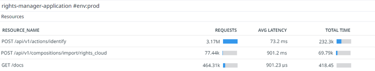
Total number of requests between 16-31 of August.

Based on the diagrams, the system was so slow in responses that we had the impression that the system was under siege!
The following sections describe how we solved the performance issue.
Spoiler alert: not a single line of code changed!
📐Understand the bottlenecks – Dive into metrics
We started digging into the Datadog log traces. We noticed that there were two patterns associated with the slow requests.
Dissecting Request Pattern #1
First, we examined the slowest request (32.1 seconds). We discovered that sending a message to an SQS took 31.7 seconds, a duration far too long for our liking. For context, the SQS is managed by AWS and it was hard to believe that a seemingly straightforward service would need 30 seconds to reply under any load.
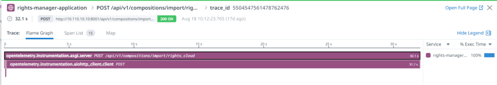
Examining slow request #1: Sending a message to an AWS SQS took 31.7 seconds
Dissecting Request Pattern #2
We examined another slow request (15.9 seconds) and the results were completely different. This time, we discovered a slow response from the database. The API call needed ~3 seconds to connect to the database and a SELECT statement on the Compositions table needed ~4 seconds. This troubled us because the SELECT query uses indexes and cannot be further optimized. Additionally, 3 seconds to obtain a database connection is really a lot.
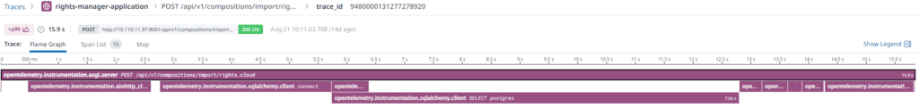
Examining a slow request #2: The database connect took 2.98 seconds and an optimized SQL-select statement took 7.13 seconds.
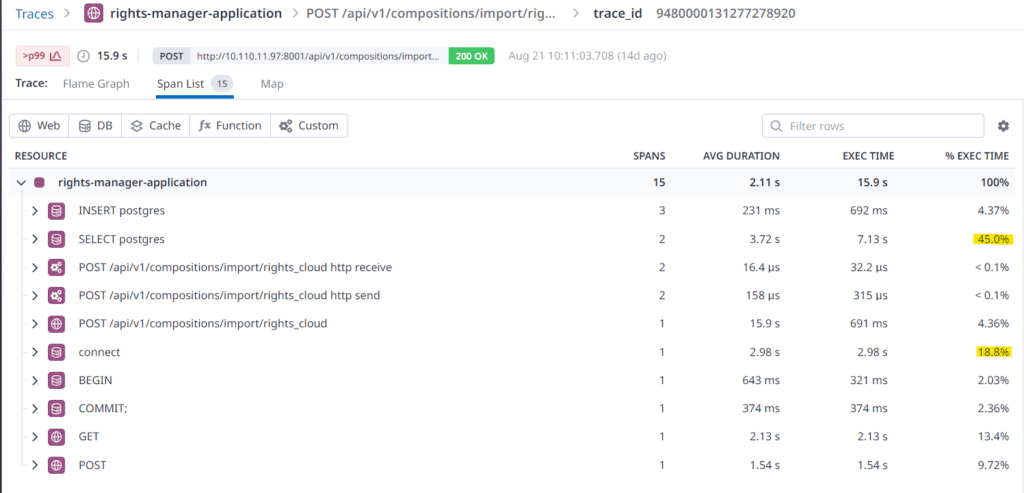
Examining a slow request #2: Dissecting the request we found that the INSERT statement was way more efficient than the SELECT statement. Also, the database connect and select took around 64% of the total request time.
Dive further into the database metrics
Based on the previous results, we started digging further into the infrastructure components.
Unfortunately, the Amazon metrics for the SQS didn’t provide us with the insight needed to understand why it was taking 30 seconds to publish a message into the queue..
So, we shifted our focus to the database metrics. Below is the diagram from AWS Database monitor.
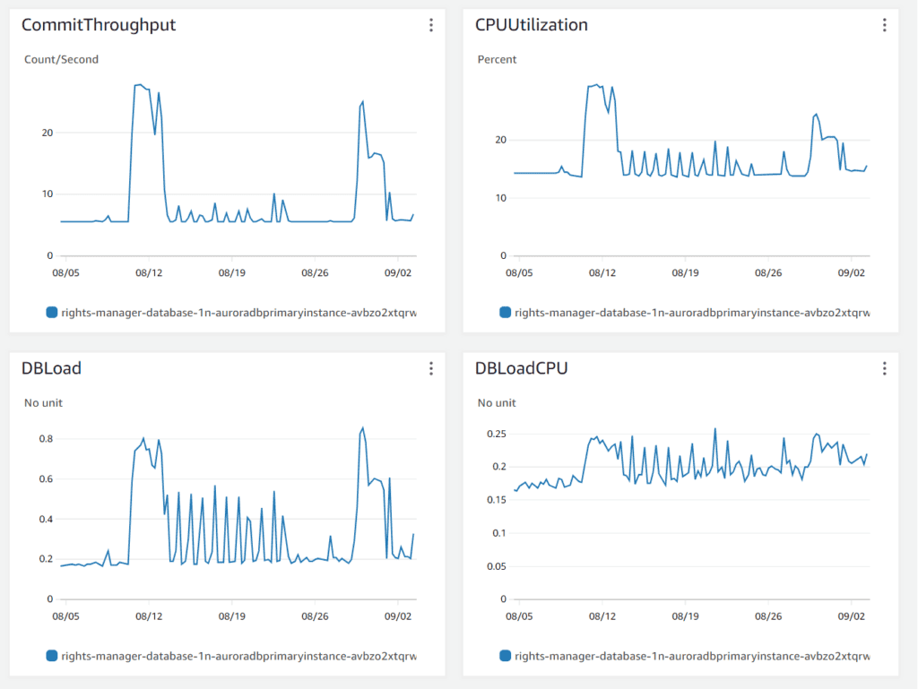
The diagram showed us that no load or latency existed on the database. The maximum load of the database was around 30%, which is relatively small. So the database connection should have been instant.
Our next move was to see if there were any slow queries. The below diagram shows the most “expensive” queries.
Once again, the result surprised us – No database load or slow query was detected from the AWS Performance Insights.
The most resource-intensive query was the intervacuum which took 0.18 of the total load, which is perfectly normal. The maximum average latency was 254 ms regarding an INSERT statement, once again reflecting perfectly normal behavior.
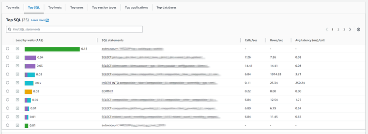
The most expensive queries that are contributing to DB load
According to AWS documentation by default, the Top SQL tab shows the 25 queries that are contributing the most to database load. To help tune your queries, the developer can analyze information such as the query text and SQL statistics.
So at that moment, we realized that the database metrics from Datadog and AWS Performance Insights were different.
The metric that solved the mystery
We suspected that something was amiss with the metrics, so we dug deeper into the system’s status when the delays cropped up. Eventually, we pinpointed a pattern: the delays consistently occurred at the start of a request batch. But here’s the twist – as time went on, the system seemed to bounce back and the delays started to taper off.
The below diagram shows that when the Rights Cloud started to send a new batch of messages around 10:07 am, the Rights Manager APIs needed more than 10 seconds to process the message in some cases.
After a while, at around 10:10 am, there was a drop in the P90 from 10 seconds to 5 seconds. Then, by 10:15 am, the P90 plummeted further to just 1 second.
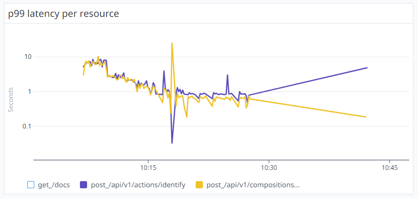
Something peculiar was afoot – instead of the usual expectation of system performance degrading over time due to heavy loads, our system was actually recovering for the same message load.
At this point, we decided to take a snapshot of the system load. And there it was – we finally made the connection!
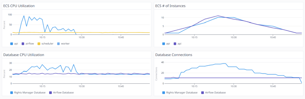
Eureka! The delays vanishes when the number of ECS (FastAPI) instances increases.
We noticed that there was a direct connection between the number of API requests and the number of ECS instances. Once the one and only ECS instance could not serve the requests, the auto scale kicked in and new ECS instances were spawned. Every ECS instance needs around 3 minutes to go live. When the instances were live, the delays decreased dramatically.
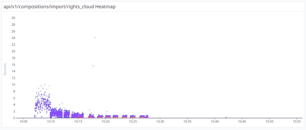
We backed up our conclusion by creating a new Datadog Heatmap. The below diagram explains the aggregation of the duration of each Import Rights Cloud Composition. It is clear, that when the 2 new FastAPI instances were spawned at 10:10 am, the delays were decreased from 10 seconds to 3 seconds. At 10:15 am there were 5 FastAPI instances and the responses dropped to 2 seconds. Around 10:30 the system spawned 10 instances and all the responses duration was around 500ms.
At the same time, the database load was stable and between 20-30%.
That was the lightbulb moment when we realized that the delays weren’t actually database or SQS related. It was the async architecture that caused the significant delays! When the ECS instance was operating at 100% and the function was getting data from the database, the SELECT query duration was in milliseconds but the function was (a)waiting for the async scheduler to resume. In reality, the function has nothing else to do but to return the results.
This explains why some functions took so much time and the metrics didn’t make any sense. Despite the SQS responding in milliseconds, the functions were taking 30 seconds because there simply wasn’t enough CPU capacity to resume their execution.
The spawn of new instances completely resolved the problem because there was always enough CPU for the async operation.
🪠Root cause
Async web servers in Python excel in performance thanks to their non-blocking request handling. This unique approach enables them to seamlessly manage incoming requests, accommodating as many as the host’s resources allow. However, unlike their synchronous counterparts, async servers lack the capability to reject new requests. Consequently, in scenarios of sustained incoming connections, the system may deplete all available resources. Although it’s possible to set a specific limit on maximum requests, determining the most efficient threshold often requires trial and error.
To broaden our understanding, we delved into the async literature and came across the Cooperative Multitasking in CircuitPython with asyncio.
Cooperative multitasking involves a programming style where multiple tasks alternate running. Each task continues until it either encounters a waiting condition or determines it has run for a sufficient duration, allowing another task to take its turn..
In cooperative multitasking, each task has to decide when to let other tasks take over, which is why it’s called “cooperative.” So, if a task isn’t managed well, it could hog all the resources. This is different from preemptive multitasking, where tasks get interrupted without asking to let other tasks run. Threads and processes are examples of preemptive multitasking.
Cooperative multitasking doesn’t mean that two tasks run at the same time in parallel. Instead, they run concurrently, meaning their executions are interleaved. This means that more than one task can be active at any given time.
In cooperative multitasking, tasks are managed by a scheduler. Only one task runs at a time. When a task decides to wait and gives up control, the scheduler picks another task that’s ready to go. It’s fair in its selection, giving every ready task a shot at running. The scheduler basically runs an event loop, repeating this process again and again for all the tasks assigned to it.
🪛Solution Approach #1
Now that we’ve identified the root cause, we’ve taken the necessary steps to address it effectively.
- Implement a more aggressive scale-out. Originally set at 50%, we’ve now set the threshold to 30% to facilitate a more responsive approach to scaling. With Amazon’s requirement of 3 minutes to spawn a new instance, the previous 1-minute timeframe for CPU reaching 100% left a mere 2-minute window of strain.
- Implement a more defensive scale in. The rule of terminating ECS instances is CPU-based. By establishing a threshold of 40% over a 2-minute interval, instances operating below 20% for the same duration trigger termination by the auto-scaler.”.
- Change the load balancer algorithm. Initially using a round-robin strategy, we encountered instances where CPU usage varied significantly, with some reaching 100% while others remained at 60%. To address this, we’ve transitioned to the “least_outstanding_requests” algorithm. This ensures that the load balancer directs requests to instances with the lowest CPU usage, optimizing performance and resource utilization across the system.
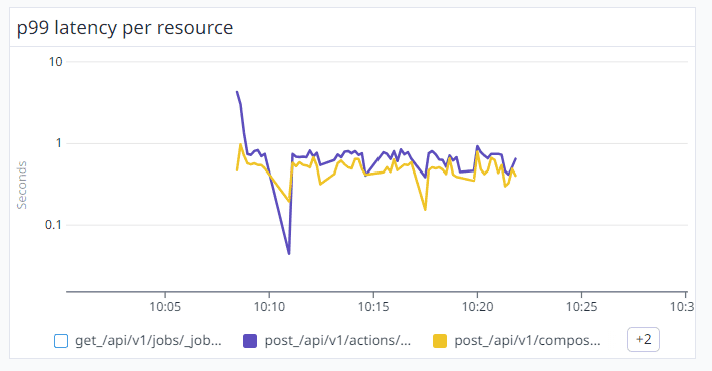
By aggressively scaling out additional ECS instances, we’ve now successfully maintained a P99 latency of under 1 second, except from the first minute of the API flood request.
🪛🪛Solution Approach #2
While the initial approach yielded results, we recognized opportunities for improvement. We proceeded with the following strategy:
- Maintain two instances at all times, allowing the system to accommodate sudden surges in API calls.
- We’ve capped the maximum ECS instances at 50.
- Implementing fine-grain logging in Datadog, to differentiate between database call durations and scheduler resumption times effectively.
🏫Lessons learned
- Understanding the implications of async architecture is crucial when monitoring system performance. During times of heavy load, processes can pause without consuming resources—a key benefit to note.
- In contrast to a non-preemptive scheduler, which switches tasks only when necessary conditions are met, preemptive scheduling allows for task interruption during execution to prioritize other tasks. Typically, processes and threads are managed by the operating system using a preemptive scheduler. Leveraging preemptive scheduling offers a promising solution to address our current challenges effectively.
- We realized that while the vCPU instances are cheap, the processing power is relatively low.
- The ECS processing power may differ between instances, while the EC2 instances provide a stable processing power.
- A FastAPI server hosted on 1 vCPU instance can handle 10K requests before maxing out CPU consumption.
- The disparity in cloud costs between completing a task in 10 hours with 1 vCPU or in 1 hour with 10 vCPUs is evident. However, from a business perspective, the substantial difference lies in completing the job 90% faster.
- A r6g.large instance typically supports approximately 1000 database connections.
🧾Conclusion
Prior familiarity with async architecture would have streamlined our approach from the start but this investigation and the results proved to be more than rewarding!
AsyncIO web servers demonstrate exceptional performance, efficiently handling concurrent requests.. However, when the system is under heavy load, the async can deplete the CPU/Memory resources in the blink of an eye! —a common challenge readily addressed by serverless architecture. With processing costs as low as €30/month for 1 vCPU & 2GB memory Fargate, implementing a proactive scaling-out strategy perfectly aligns with business objectives.